In the previous article, we discussed the Continuity equation, and the rate of flow discharge In Fluid Mechanics, the hardy cross method is used to analyse the Pipe network with help of a continuity equation.

Pipe Network
A pipe network is an interconnected system of pipes forming several loops or circuits. The pipe network is shown in the following figure.
Examples of such networks of pipes are the municipal water distribution systems in cities and laboratory supply systems. In such system, it is required to determine the distribution of flow through the various pipes of the network. The following are the necessary conditions for any network of pipes :
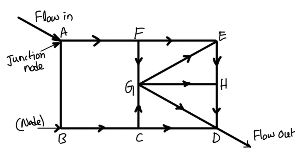
(ABCGFA, FEGF, GEHG, GHDG and GCDG are the different loops from the above pipe network)
- The flow into each junction must equal the flow out of the junction. This is due to the continuity equation.
- The algebraic sum of head losses around each loop must be zero. This means that in each loop, the loss of head due to flow in a clockwise direction must be equal to the loss of head due to flow in an anticlockwise direction.
- The head loss in each pipe is expressed as hf =r Qn. The value of r depends upon the length of the pipe, the diameter of the pipe and the coefficient of friction of the pipe. The value of n for turbulent flow is 2. We know that
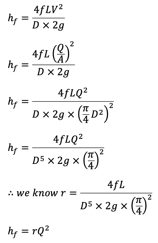
This head loss will be positive when the pipe is a part of the loop and the flow in the pipe is clockwise. Generally, pipe network problems are difficult to solve analytically. Hence the methods of successive approximations are used. ‘Hardy Cross Method’ is one such method which is commonly used to analyze the pipe networks.
Hardy Cross Method
The procedure for Hardy Cross Method is as follows :
- In this method, a trial distribution of discharges is made arbitrary but in such a way that the continuity equation is satisfied at each junction (or node).
- With the assumed values of Q, the head loss in each pipe is calculated according to equation (a).
- Now consider any loop (or circuits). The algebraic sum of head losses around each loop must be zero. This means that in each loop, the loss of head due to flow in the clockwise direction must be equal to the loss of head due to flow in the anticlockwise direction.
- Now calculate the net head loss around each loop considering the head loss to be positive in clockwise flow and to be negative in anticlockwise flow.
If the net head loss due to assumed values of Q round the loop is zero, then the assumed values of Q in that loop is correct. But if the net head loss due to assumed values of Q is not zero, then the assumed Q values are corrected by introducing a correction AQ for the flows until the circuit is balanced.
Let us take
Q0 = Assumed discharge
Q = Correct Discharge
Q = Q0 + ∆Q
Head loss for the pipe will be
hf = rQ2
hf = r(Q0 + ∆Q)2
For the complete network of pipes, the total head loss we can write as follows,
Σhf = Σ(rQ2)
Σhf = Σ r(Q0 + ∆Q)2
Σhf = Σ r(Q02 + ∆Q2+2 Q0 × ∆Q)
As the ∆Q is very small, so ∆Q2 can also be neglected
Σhf = Σ r(Q02 + 2 Q0 × ∆Q)
Σhf = ΣrQ02 + Σr × 2Q0∆Q
For the correct distribution, the net headloss should be zero, so Σhf must be 0, we can equate the above equation to zero, and we get
ΣrQ02 + Σr × 2Q0∆Q = 0
ΣrQ02 + ∆Q Σr 2Q0 = 0
∆Q can be taken out from the above relation since it will be same for the one circuit of the pipe network, we can re-write the above relation as follows
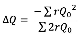
We can re-write the ∆Q as the correction factor for the entire network, then the above relation becomes as follows
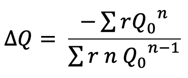
For turbulent flow, the value of n = 2 and hence the above correction factor becomes as

- If the value of ∆Q comes out to be positive, then it should be added to the flows in the clockwise direction (he flows in clockwise direction in a loops are considered positive) and subtracted from the flows in the anticlockwise direction.
- Some pipes may be common to two circuits (or two loops), then the two corrections are applied to these pipes.
- After the corrections have been applied to each pipe in a loop and to all loops, a second trial calculation is made for all loops. The procedure is repeated till AQ becomes negligible.
Example problem on Hardy Cross Method
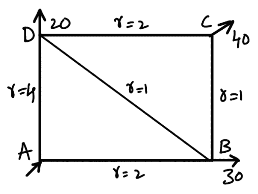
Problem Statement: Calculate the discharge in each pipe of the network shown in the following figure. The pipe network consists of 5pipes. The head loss h, in a pipe is given by hf = r Q2 . The values of r for various pipes and also the inflow or outflows at nodes are shown in the figure.
Answer:
Inflow at node A = 90, outflow at B = 30, at C = 40 and at D = 20.
Values of r for AB = 2, for BC = 1, for CD = 2, for AD = 4 and for BD = 1.
First Trail using the Hardy Cross Method
For the first trial, the discharges are assumed as shown in the following figure (a) so that continuity is satisfied at each node (i.e., flow into a node = flow out of the node).
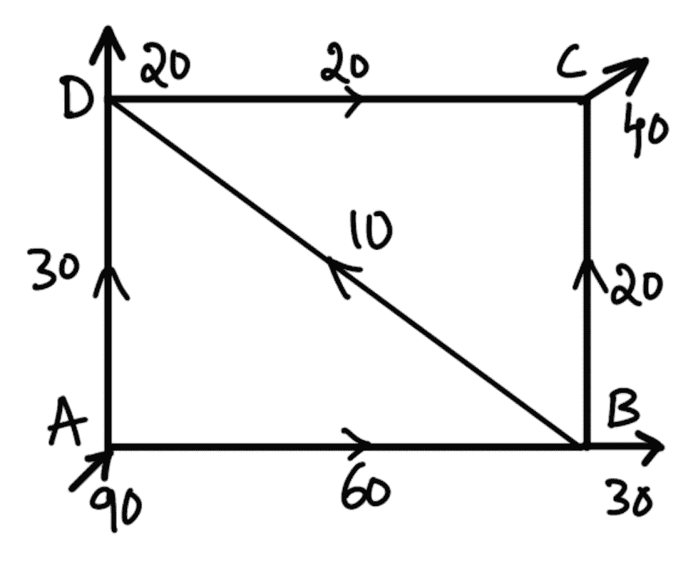
For this distribution of discharge, the corrections ∆Q for the loops ABD and BCD are calculated.
| Loop | ADB | | | |
| Pipe | r | Q0 | hf = rQ02 | 2rQ0 |
| AD | 4 | 30 | 4×302 =3600 | 2×4×30 =240 |
| DB | 1 | 10 | -1×102 =-100 | 2×1×10 =20 |
| AB | 2 | 60 | -2×602 =-7200 | 2×2×60 =240 |
| | | | ΣrQ02 =-3700 | Σ2rQ0 =500 |
| | | ∆Q = | -(-3700)/500 | |
| | | ∆Q = | 7.4 | |
In the loop ADB, the head loss hf is negative in pipes DB and AB as the direction of discharges in these pipes is anticlockwise.
As ∆Q is positive for loop AB, hence it should be added to the flow in the clockwise direction and subtractedfrom the flow in the anticlockwise direction. Hence the corrected flow for second trial for loop ADB will be as follows :
Pipe AD = 30 + 7.4 = 37.4 (flow is clockwise)
Pipe AB = 60 – 7.4 = 52.6 (flow is anticlockwise)
Pipe BD = 10 – 7.4 = 2. 6 (flow is anticlockwise)
| Loop | DCB | | | |
| Pipe | r | Q0 | hf = rQ02 | 2rQ0 |
| DC | 2 | 20 | 2×202 =800 | 2×2×20 =80 |
| CB | 1 | 20 | -1×202 =-400 | 2×1×20 =40 |
| BD | 1 | 10 | 1×102 =100 | 2×1×10 =20 |
| | | | ΣrQ02 =500 | Σ2rQ0 =140 |
| | | ∆Q = | –500/130 | |
| | | ∆Q = | -3.57 | |
The head loss in pipe BC for loop CB is negative as the direction of discharge in pipe BC in anticlockwise.
As ∆Q is negative for loop CB, hence it should be subtracted from the flow in the clockwise direction and added to the flow in the anticlockwise direction. Hence corrected flow for second trial for loop DCB will be as follows :
Pipe DC = 20 – 3.6 = 16.4
Pipe BC = 20 + 3.6 = 23.6
Pipe BD* = 2.6 -36 = -1
Note: The pipe BD is common to two loops (i.e., loop AB and loop DCB). Hence this pipe will get two corrections. After the two corrections, the resultant flow in pipe BD is negative in loop DC. Hence the direction of flow will be anticlockwise in pipe BD for loop DCB.
Second Trail using the Hardy Cross Method
The distribution of discharges in various pipes for second trial is shown in the following figure (b).
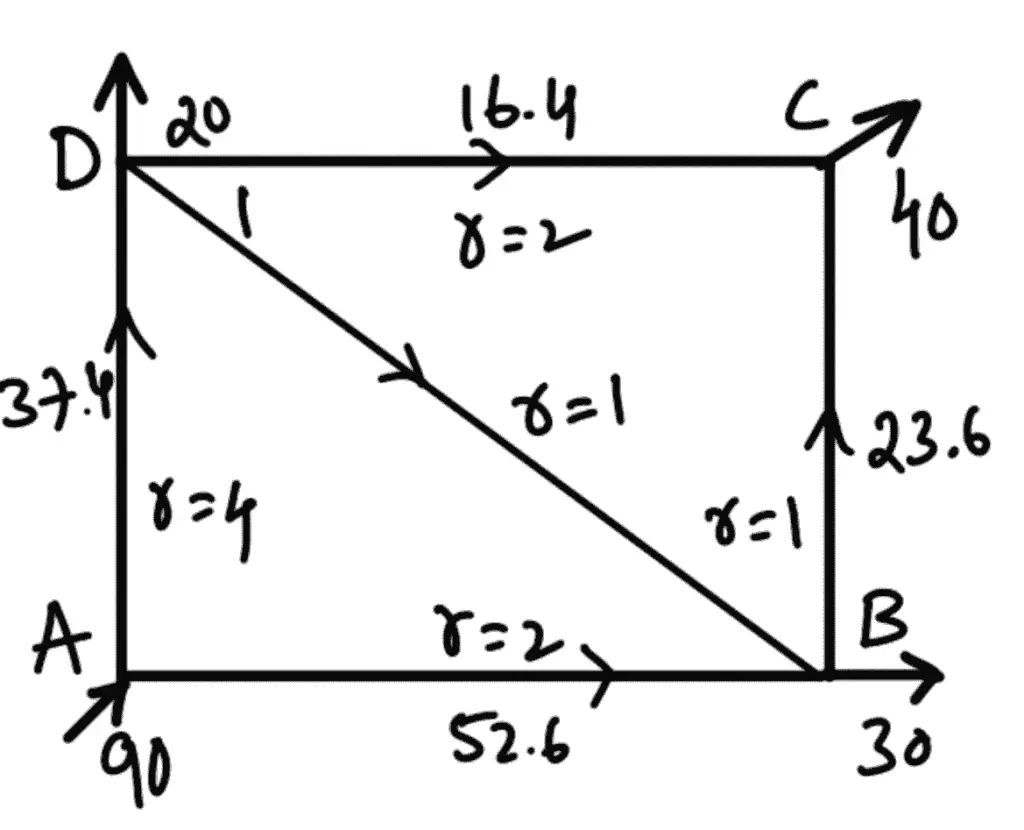
For second trial the correction ∆Q for loops ADB and DC are calculated as follows:
For this distribution of discharge, the corrections ∆Q for the loops ABD and BCD are calculated.
| Loop | ADB | | | |
| Pipe | r | Q0 | hf = rQ02 | 2rQ0 |
| AD | 4 | 37.4 | 4×37.42 =5595 | 2×4×37.4 =299.2 |
| DB | 1 | 1 | 1×12 =1 | 2×1×1 =2 |
| AB | 2 | 52.6 | -2×52.62 =-5533.3 | 2×2×52.6 =210.4 |
| | | | ΣrQ02 =62.54 | Σ2rQ0 =511.6 |
| | | ∆Q = | -62.54/511.6 | |
| | | ∆Q = | -0.122 | (~ -0.1) |
As ∆Q is negative, hence it should be subtracted from the flow in the clockwise direction and added to the flow in the anticlockwise direction
As the correction (∆Q) is small (i.e., ∆Q = 0.1), this correction is applied and further trials are discontinued.
Hence corrected flow for loop ADB will be as follows :
For pipe AD, Q0 = 37.4 – 0.1 = 37.3 (as flow is clockwise)
For pipe DB, Q0 = 1 – 0.1 = 0.9 (as flow is clockwise)
For pipe AB, Q0 = 52.6 + 0.1 = 52.7 (as flow is anti clockwise)
| Loop | DCB | | | |
| Pipe | r | Q0 | hf = rQ02 | 2rQ0 |
| DC | 2 | 16.4 | 2×16.42 =537.9 | 2×2×16.4 =65.6 |
| CB | 1 | 23.6 | -1×23.62 =-556.9 | 2×1×23.6 =47.2 |
| BD | 1 | 1 | -1×12 =-1 | 2×1×11 =2 |
| | | | ΣrQ02 =-20 | Σ2rQ0 =114.8 |
| | | ∆Q = | -(-20)/114.8 | |
| | | ∆Q = | 0.174 | (~0.2) |
As AQ is positive, hence it should be added to the flow in the clockwise direction and subtracted from the flow in the anticlockwise direction.
As the correction (∆Q) is small (i.e., ∆Q = 0.2), this correction is applied and further trials are discontinued
Hence corrected flow for loop DCB will be as follows :
For pipe DC, Q0 = 16.4 + 0.2 = 16.6 (clockwise flow)
For pipe CB, Q0 = 23.6 – 0.2 = 23.4 (anticlockwise flow)
For pipe BD, Q0 = 0.9 – 0.2 = 0.7 (anticlockwise flow)
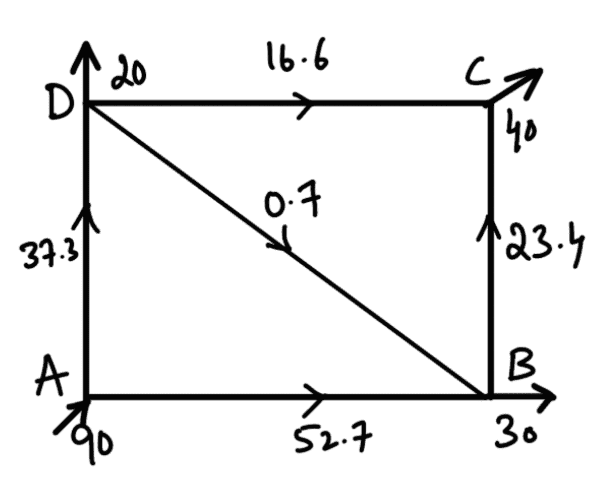
The final distribution of discharges in each pipe is as follows :
Discharge in pipe
AD = 37.3 from A to D
AB = 52.7 from A to B
DB = 0.7 from D to B
DC = 16.6. from D to C
BC = 23.4 from B to C
The final discharge in each pipe is shown in the following figure(c)
Note: The pipe DB is common to two loop (i.e., loops ADB and loop DBC). Hence this pipe will get two corrections. For loop ADB, the correction ∆Q = 0.1 and hence the corrected flow in pipe DB is 1 – 0.1 = 0.9. Now again, the correction is applied to pipe DB when we consider loop BC. For loop DBC, the correction ∆Q = 0.2 but flow is anticlockwise and hence the final correct flow in pipe DB will be 0.9 – 0.2 = 0.7.
This is how we can calculate the discharge in each pipe of the given pipe network using the Hardy Cross Method procedure. Let us know what you think about this article in the comment sectio below.

Leave a Reply