Project Title: Prediction And Performance Analysis Of 30kW Solar Pv System Using Machine Learning Linear Regression Algorithm
The Final Year Project on “Prediction And Performance Analysis Of 30kW Solar Pv System Using Machine Learning Linear Regression Algorithm” submitted by Kowsika NP (from Alagappa Chettiar Government College Of Engineering And Technology, karaikudi) to extrudesign.com.
ABSTRACT
The global shift towards renewable energy sources (RES) has driven the development of photovoltaic (PV) panels. For example, the costs of producing electricity from PV panels have dropped significantly, while simultaneously increasing the energy conversion efficiency. However, since PV panel energy output depends on weather conditions such as cloud cover and solar irradiance, the energy output of the PV panels is unstable. Although ML techniques are nothing new, the improved computational capacity and the higher availability of quality data have made the techniques useful for forecasting. Forecasting solar energy is becoming an important issue in the context of renewable energy sources and Machine Learning Algorithms play an important role in this field.
While low-cost energy storage will help solar power become more ubiquitous and dispatchable, forecasting remains a cost-effective tool to integrate solar into the grid, since it doesn’t require capital expenditure for permits and equipment. What’s more, operating grid-connected batteries economically will require accurate forecasts of solar variability to select the charging strategy that takes maximum advantage of the available solar power and avoids undue cycling of the energy storage system.
Our main aim is to predict and analyze the performance of a 30Kw solar grid using a linear regression machine learning algorithm. By predicting the electrical output we will be able to connect loads according to the electrical output. In this project, we took solar irradiance and Temperature to analyze the performance of the solar grid. The performance is analyzed with performance indices- RMSE(Root Mean Squared Error), MAE(Mean Absolute Error), MSE(Mean Squared Error).
1. INTRODUCTION
1.1 INTRODUCTION OF PROJECT ON ANALYSIS OF 30KW SOLAR PV SYSTEM
Besides direct heating of the Earth’s surface, solar irradiation brings about the constant renewal of wind energy, tidal and wave power, hydropower, and the ocean’s natural thermal gradient. Solar energy is more than enough to meet all the energy needs worldwide. To a greater or lesser extent, solar energy is available in every country of the world. Since the outbreak of the world energy crisis in 1973, the use of solar energy for the production of thermal and electrical energy has been constantly in the focus of attention. The use of solar energy contributes to the greenhouse gas emissions reduction, fossil fuel consumption decrease, development of the local industry.
Over recent years there has been a constant increase of the investment in the research of photovoltaic conversion of solar radiation to produce high quality, yet cheap solar cells and other components of the photovoltaic systems. Numerous companies and organizations compete in the promotion and production of photovoltaic systems. Up to now, several thousands of solar PV plants of 1 kW to several hundreds of megawatts have been installed worldwide.
Solar power forecasting is the process of gathering and analyzing data to predict solar power generation on various time horizons to mitigate the impact of solar intermittency. Solar power forecasts are used for efficient management of the electric grid and power trading.
Prediction and performance analysis of solar PV systems is done by means of machine learning. Since machine learning needs no human intervention and easily identifies trends and patterns.
1.2 OBJECTIVE OF ANALYSIS OF 30KW SOLAR PV SYSTEM
By predicting the electrical output we will be able to connect loads according to the electrical output. However, since PV panel energy output depends on weather conditions such as cloud cover and solar irradiance, the energy output of the PV panels is unstable.
Our main objective of the project is, Prediction and performance analysis of the 30 kW solar PV system installed in our department is done by linear regression machine algorithm.
1.3 PROBLEM STATEMENT
Solar power output highly depends on weather conditions. solar panels are more productive when temperatures are low. High temperatures reduce the power output of the PV cells due to voltage drop. Thus, a cool sunny day is a lot better condition for the optimal functioning of the solar panels.
By analyzing the performance of the solar PV system according to the temperature we will predict the effective electrical output.
2. LITERATURE SURVEY
2.1 LITERATURE SURVEY ON ANALYSIS OF 30KW SOLAR PV SYSTEM USING MACHINE LEARNING
Dastan Hussen Maulud , Adnan Mohsin Abdulazeez (2016)
One of the most common and comprehensive statistical and machine learning algorithms is linear regression. Linear regression is used to find a linear relationship between one or more predictors. Linear regression has two types: simple regression and multiple regression (MLR).
This paper discusses various works by different researchers on linear regression and polynomial regression and compares their performance using the best approach to optimize prediction and precision. Almost all of the articles analyzed in this review are focused on datasets; to determine a model’s efficiency, it must be correlated with the actual values obtained for the explanatory variables.
Suneel Raju Penderm, Suresh Mikkili(2021)
The main design objective of the solar photovoltaic (PV) systems is to extract the maximum power from the PV systems for a long time. The amount of power extracted from the PV array can be affected by temperature, solar irradiation, dust accumulation, wind speed, PV array configuration, and shading pattern. Often, the PV arrays are completely or partially shadowed and have been recognized as a major challenging concern which can reduce the output power of PV arrays due to mismatching power loss between the PV modules and also represents multiple Maximum PowerPoints (MPPs) in the electrical characteristics (I–V and P–V characteristics).
Rajib Baran Roy1 , MD. Rokonuzzaman, Nowshad Amin, Saifur Rahman(2021)
A comparative analysis among the algorithms in terms of the performance of handling the trained dataset is presented. The MATLAB/Simulink environment is used to design the maximum power point tracking energy harvesting system and the artificial neural network toolbox is utilized to analyze the developed model. The proposed model is trained with 1000 datasets of solar irradiance, temperature, and voltages. Seventy percent of data is used for training, while 15% of data is employed for validation, and 15% of data is utilized for testing. The trained datasets error histogram represents zero error in the training, validation, and test phase of data matching.
Dragana D. Milosavljević ,Tomislav M. Pavlović , Danica S. Piršl
The article presents basic data on a 2 kW solar PV plant installed on the building of the Faculty of Sciences and Mathematics and the equipment for the estimation of its performance and energy efficiency depending on the real climate conditions (inverter, communication system, automatic meteorological station, etc.). The article aims to apply the obtained results in the integration of solar energy generation into a transmission network to increase the use of solar PV plants for commercial purposes in Serbia.
Emil Isaksson , Mikael Karpe Conde (2018)
The increased competitiveness of solar PV panels as a renewable energy source has increased the number of PV panel installations in recent years. In the meantime, higher availability of data and computational power have enabled machine learning algorithms to perform improved predictions. As the need to predict solar PV energy output is essential for many actors in the energy industry, machine learning and time series models can be employed towards this end.
3. PROPOSED SYSTEM
3.1 BLOCK DIAGRAM OF 30kW SOLAR PV SYSTEM
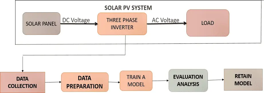
3.2 BLOCK DIAGRAM EXPLANATION
- In a solar PV system, DC power output is obtained from the solar panels. In order to supply the supply load, DC output is converted into AC by means of an inverter.
- From the inverter, AC output is given to distributed loads
- In order to train the model, data required to train the model is collected from the inverter.
- The model will train to analyze and predict the output power for the input we gave.
4. SOLAR PV SYSTEM
4.1 OVERVIEW
A photovoltaic (PV) system is composed of one or more solar panels combined with an inverter and other electrical and mechanical hardware that use energy from the Sun to generate electricity. PV systems can vary greatly in size from a small rooftop or portable systems to massive utility-scale generation plants.
4.2 WORKING
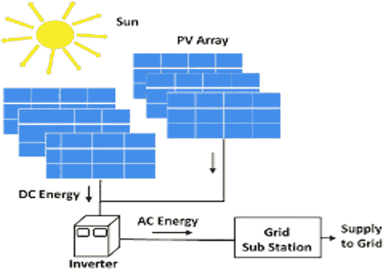
The light from the Sun is made up of packets of energy called photons, falls onto a solar panel, and creates an electric current through a process called the photovoltaic effect. Each panel produces a relatively small amount of energy but can be linked together with other panels to produce higher amounts of energy as a solar array. The electricity produced from a solar panel (or array) is in the form of direct current (DC). Although many electronic devices use DC electricity, including your phone or laptop, they are designed to operate using the electrical utility grid which provides (and requires) alternating current (AC). Therefore, for solar electricity to be useful it must first be converted from DC to AC using an inverter. This AC electricity from the inverter can then be used to power electronics locally, or be sent on to the electrical grid.
4.3 COMPONENTS
4.3.1 SOLAR PANEL
A solar panel consists of many solar cells with semiconductor properties encapsulated within a material to protect it from the environment. These properties enable the cell to capture light, or more specifically, the photons from the sun, and convert their energy into useful electricity through a process called the photovoltaic effect. On either side of the semiconductor is a layer of conducting material which “collects” the electricity produced.
4.3.2 INVERTER
An inverter is an electrical device that accepts electrical current in the form of direct current (DC) and converts it to alternating current (AC). For solar energy systems, this means the DC from the solar array is fed through an inverter which converts it to AC. This conversion is necessary to operate most electric devices or interface with the electrical grid.
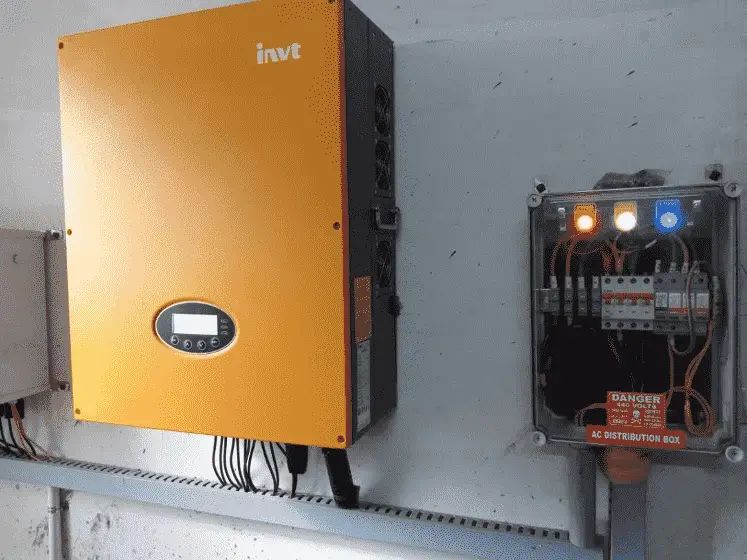
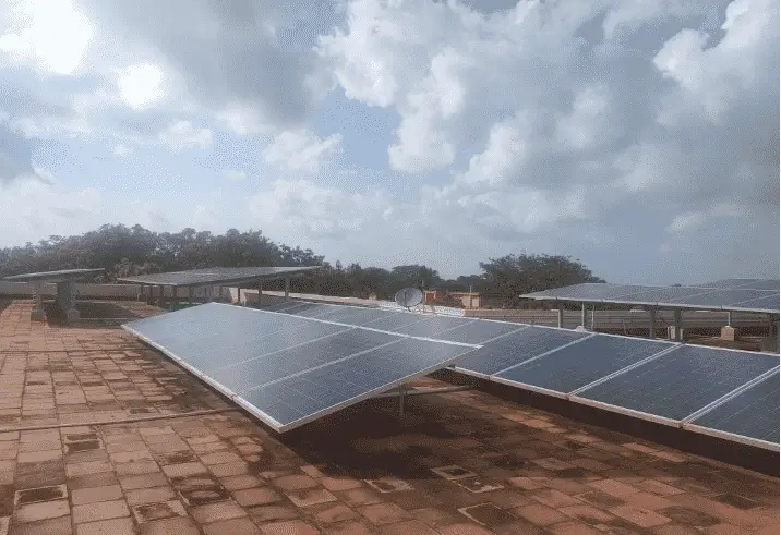
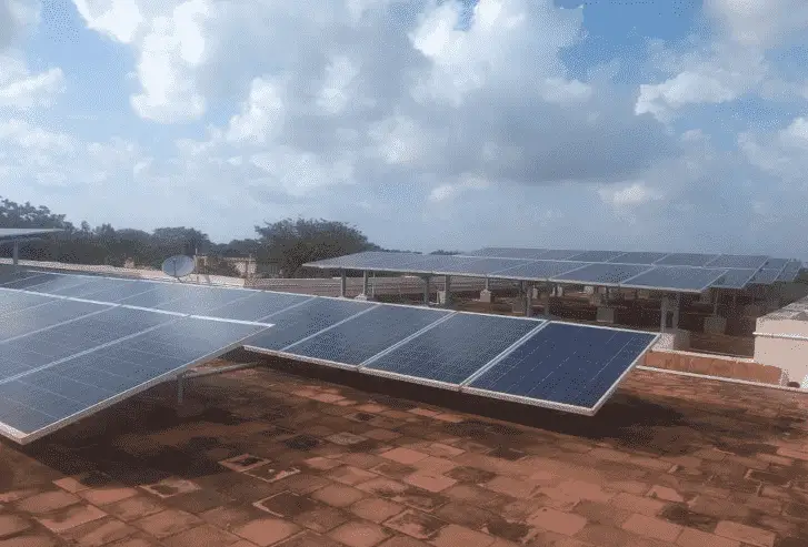
4.4 SOLAR PV SYSTEM IN OUR DEPARTMENT 4.4.1 SOLAR PANEL
4.4.1. Solar Panel
4.4.2 SOLAR PANEL SPECIFICATION
| Maximum Power (watt) | 325 |
| Open Circuit Voltage(volt) | 46 |
| Short Circuit Current (amp) | 9.25 |
| Maximum Point Voltage(volt) | 37.1 |
| Maximum Point Current (Amp) | 8.77 |
| Maximum Series Fuse(Amp) | 15 |
| Maximum System Voltage(volt) | 1000 |
| Output Power(watt) | -0/+4.99w |
| STC | 1000W/M square, AM 1.5, 25 degree Celsius |
4.4.3 Data Collected
| Irradiance | Temperature | Output Power |
| (Wm-2) | (ºC) | (kW) |
| 549.23 | 30.94 | 13.1 |
| 555.13 | 31.18 | 12.52 |
| 557.1 | 31.43 | 11.93 |
| 561.04 | 31.67 | 13.35 |
| 564.97 | 31.91 | 14.77 |
| 597.29 | 32.12 | 15.15 |
| 629.62 | 32.34 | 15.53 |
| 661.94 | 30.98 | 18.48 |
| 694.26 | 32.76 | 21.42 |
| 660.65 | 32.91 | 22.87 |
| 627.05 | 33.06 | 24.32 |
| 593.44 | 33.2 | 23.37 |
| 559.83 | 33.35 | 22.42 |
| 545.5 | 33.43 | 22.67 |
| 531.17 | 33.5 | 22.91 |
| 516.83 | 33.58 | 23.16 |
| 502.5 | 33.65 | 23.4 |
| 458.12 | 28.13 | 18.91 |
| 413.74 | 27.32 | 14.43 |
| 369.36 | 22.01 | 9.94 |
| 324.98 | 20.98 | 5.45 |
| 280.37 | 23.89 | 9.66 |
| 235.75 | 26.8 | 13.86 |
| 191.14 | 29.7 | 12.22 |
| 146.52 | 32.61 | 10.58 |
| 114.91 | 21.65 | 7.42 |
| 83.31 | 20.13 | 4.25 |
| 912.84 | 28.98 | 19.12 |
| 904.7 | 29.97 | 19.98 |
| 896.56 | 30.96 | 20.83 |
| 888.41 | 31.95 | 21.29 |
| 880.27 | 32.94 | 22.36 |
| 839.41 | 33.01 | 22.97 |
| 798.56 | 33.09 | 24.12 |
| 757.7 | 33.16 | 25.28 |
| 716.84 | 33.23 | 26.04 |
| 528.37 | 33.05 | 23.4 |
| 481.6 | 30.5 | 21.32 |
| 434.84 | 27.95 | 19.24 |
| 388.07 | 25.39 | 12.2 |
| 341.3 | 22.84 | 5.15 |
| 295.92 | 24.16 | 9.51 |
| 250.54 | 23.5 | 13.86 |
| 205.15 | 26.04 | 12.27 |
| 159.77 | 24.15 | 10.68 |
| 125.23 | 23.91 | 7.47 |
| 90.7 | 22.77 | 4.25 |
| 615.98 | 27.15 | 19.46 |
| 593.28 | 28.38 | 20.19 |
| 570.57 | 29.62 | 20.91 |
| 547.87 | 30.85 | 21.69 |
| 525.16 | 32.08 | 22.47 |
| 538.22 | 32.27 | 21.91 |
| 551.27 | 32.46 | 21.34 |
| 564.33 | 32.64 | 22.09 |
| 577.38 | 32.83 | 22.83 |
| 369.14 | 30.25 | 19.71 |
| Irradiance | Temperature | Output Power |
| (Wm-2) | (ºC) | (kW) |
| 333.36 | 26.52 | 12.99 |
| 297.59 | 23.55 | 6.27 |
| 261.81 | 26.35 | 11.39 |
| 226.03 | 28.52 | 16.51 |
| 185.96 | 27.99 | 15.4 |
| 145.9 | 27.45 | 14.28 |
| 105.83 | 26.31 | 12.32 |
| 65.76 | 25.05 | 10.35 |
| 52.37 | 23.99 | 9.19 |
| 38.99 | 39.36 | 8.03 |
| 795.07 | 32.98 | 23.38 |
| 800.07 | 32.54 | 22.76 |
| 805.06 | 30.89 | 21.54 |
| 810.06 | 32.24 | 22.01 |
| 815.05 | 33.59 | 22.49 |
| 802.26 | 33.61 | 22.54 |
| 789.47 | 33.64 | 21.59 |
| 776.68 | 33.66 | 23.08 |
| 763.89 | 33.68 | 23.58 |
| 725.51 | 32.09 | 24.12 |
| 687.12 | 30.5 | 24.66 |
| 648.74 | 30.12 | 20.41 |
| 610.36 | 27.32 | 16.16 |
| 571.97 | 24.05 | 14.3 |
| 533.59 | 22.52 | 12.44 |
| 495.2 | 21.36 | 10.59 |
| 456.82 | 32.24 | 8.73 |
| 409.21 | 32.01 | 8.74 |
| 361.61 | 31.77 | 8.75 |
| 314 | 31.54 | 7.8 |
| 266.39 | 31.3 | 6.85 |
| 230.06 | 31.06 | 6.09 |
| 193.74 | 30.82 | 5.33 |
| 157.41 | 30.58 | 4.96 |
| 121.08 | 30.34 | 4.58 |
| 52.37 | 29.88 | 4.4 |
| 38.99 | 29.43 | 4.21 |
| 513.92 | 30.49 | 3.53 |
| 458.4 | 30.42 | 3.87 |
| 402.88 | 30.34 | 4.21 |
| 346.3 | 30.19 | 4.04 |
| 289.72 | 30.04 | 3.87 |
| 233.13 | 29.88 | 3.48 |
| 176.55 | 29.73 | 3.1 |
| 136.54 | 29.43 | 2.81 |
| 93.53 | 24.31 | 2.53 |
| 622.9 | 31.51 | 8.46 |
| 566.19 | 31.39 | 8.03 |
| 509.48 | 31.27 | 7.6 |
| 452.76 | 31.15 | 7.53 |
| 396.05 | 31.03 | 7.46 |
| 336.94 | 30.84 | 7.02 |
| 277.84 | 30.64 | 6.58 |
| 336.94 | 30.84 | 7.02 |
| 277.84 | 30.64 | 6.58 |
| 218.73 | 30.45 | 5.46 |
| 159.62 | 30.25 | 4.33 |
| Irradiance | Temperature | Output Power |
| (Wm-2) | (ºC) | (kW) |
| 98.1 | 23.81 | 3.76 |
| 86.86 | 22.45 | 3.18 |
| 523.27 | 29.14 | 15.96 |
| 471.24 | 29.03 | 17.77 |
| 419.2 | 28.93 | 19.58 |
| 367.17 | 28.82 | 12.35 |
| 315.13 | 28.71 | 5.61 |
| 267.76 | 28.55 | 4.53 |
| 220.4 | 28.39 | 3.45 |
| 173.03 | 28.22 | 6.13 |
| 125.66 | 28.06 | 8.82 |
| 97.14 | 27.81 | 8.12 |
| 68.61 | 27.56 | 7.41 |
| 465.18 | 31.28 | 11.43 |
| 423.52 | 31.17 | 11.37 |
| 381.85 | 31.06 | 11.3 |
| 340.19 | 30.95 | 10.1 |
| 298.52 | 30.84 | 10.14 |
| 250.24 | 30.59 | 11.9 |
| 201.96 | 30.35 | 16.36 |
| 153.67 | 30.1 | 5.97 |
| 105.39 | 29.85 | 11.51 |
| 81.59 | 25.51 | 7.96 |
| 85.8 | 26 | 4.4 |
| 454.32 | 30.51 | 10.59 |
| 411.38 | 30.38 | 13.7 |
| 368.44 | 30.26 | 14.61 |
| 325.5 | 30.13 | 14.5 |
| 282.56 | 30 | 10.14 |
| 236.97 | 29.75 | 6.75 |
| 191.38 | 29.49 | 4.9 |
| 168.58 | 29.36 | 3.61 |
| 100.19 | 28.98 | 3.37 |
| 76.85 | 26.56 | 3.07 |
| 53.5 | 24.13 | 2.86 |
| 373.51 | 23.58 | 4.92 |
| 334.84 | 23.52 | 8.56 |
| 296.18 | 23.46 | 5.45 |
| 257.51 | 23.4 | 1.63 |
| 218.84 | 23.34 | 1.63 |
| 187.8 | 23.25 | 1.33 |
| 156.75 | 23.15 | 1.28 |
| 125.71 | 23.06 | 1.23 |
| 94.66 | 22.96 | 1.8 |
| 73.5 | 23.47 | 1.78 |
| 52.33 | 23.98 | 2.51 |
| 472.16 | 25.39 | 7.21 |
| 428.98 | 25.33 | 6.77 |
| 385.81 | 25.26 | 6.65 |
| 342.63 | 25.2 | 6.78 |
| 299.45 | 25.13 | 6.09 |
| 250.22 | 25.08 | 4.49 |
| 200.98 | 25.03 | 11.2 |
| 151.75 | 24.97 | 8.25 |
| 102.51 | 24.92 | 5.29 |
| 54.53 | 24.66 | 4.04 |
| 78.52 | 25.1 | 6.73 |
- Nearly 170 data sets were collected. Output power is collected from the inverter of the 30kW solar PV system installed in our campus
- Irradiance and Temperature were collected from NASA with data on the same dates as output power were collected
5. MACHINE LEARNING
5.1 DEFINITION OF MACHINE LEARNING
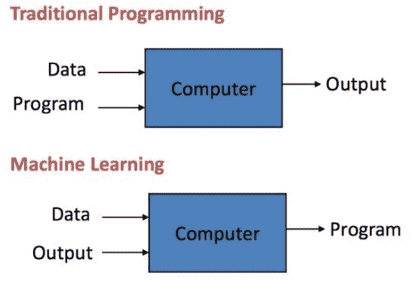
Machine Learning is getting computers to program themselves. If programming is automation, then machine learning is automating the process of automation.
5.2 KEY ELEMENTS
Every machine learning algorithm has three components:
- Representation: how to represent knowledge. Examples include decision trees, sets of rules, instances, graphical models, neural networks, support vector machines, model ensembles and others.
- Evaluation: the way to evaluate candidate programs (hypotheses). Examples include accuracy, prediction and recall, squared error, likelihood, posterior probability, cost, margin, entropy k-L divergence and others.
- Optimization: the way candidate programs are generated known as the search Sprocess. For example combinatorial optimization, convex optimization, constrained optimization.
5.3 TYPES OF LEARNING
- Supervised learning: (also called inductive learning) Training data includes desired outputs. This is spam this is not, learning is supervised.
- Unsupervised learning: Training data does not include desired outputs.Example is clustering. It is hard to tell what is good learning and what is not.
- Semi-supervised learning: Training data includes a few desired outputs.
- Reinforcement learning: Rewards from a sequence of actions. AI types like it,it is the most ambitious type of learning.
- Classification: when the function being learned is discrete.
- Regression: when the function being learned is continuous.
- Probability Estimation: when the output of the function is a probability.
5.4 LINEAR REGRESSION
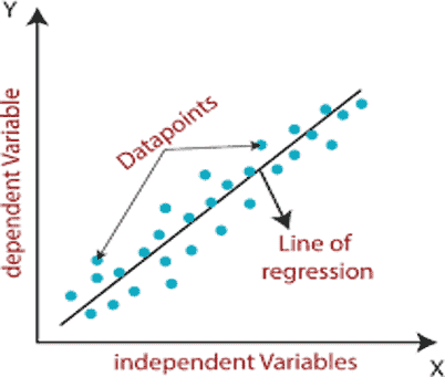
Linear regression is a linear model that assumes a linear relationship between the input variables (x) and the single output variable (y). More specifically, that y can be calculated from a linear combination of the input variables (x).
It involves graphing a line over a set of points.
5.5 LINEAR REGRESSION MODEL REPRESENTATION
The representation is a linear equation that combines a specific set of input values (x) the solution to which is the predicted output for that set of input values (y). As such, both the input values (x) and the output value are numeric.
The linear equation assigns one scale factor to each input value or column, called a coefficient, and represented by the capital Greek letter Beta (B). One additional coefficient is also added, giving the line an additional degree of freedom (e.g. moving up and down on a two-dimensional plot) and is often called the intercept or the bias coefficient.
For example, in a simple regression problem (a single x and a single y), the form of the model would be:
y = b0 + b1*x ……. (1)
The values b0 and b1 must be chosen so that they minimize the error. If the sum of squared error is taken as a metric to evaluate the model, then the goal to obtain a line that best reduces the error

…….(2)
In higher dimensions when we have more than one input (x), the line is called a plane or a hyper-plane. The representation, therefore, is in the form of the equation and the specific values used for the coefficients (e.g. b0 and b1 in the above example)
Linear regression refers to the number of coefficients used in the model. The formula for coefficient,

………. (3)
When a coefficient becomes zero, it effectively removes the influence of the input variable on the model and therefore from the prediction made from the model (0 * x = 0). This becomes relevant if you look at regularization methods that change the learning algorithm to reduce the complexity of regression models by putting pressure on the absolute size of the coefficients, driving some to zero.
In our project, we take
Independent variable – Irradiance, Temperature
Dependent variable – Output power
6 SIMULATION RESULT
6.1 FLOW CHART
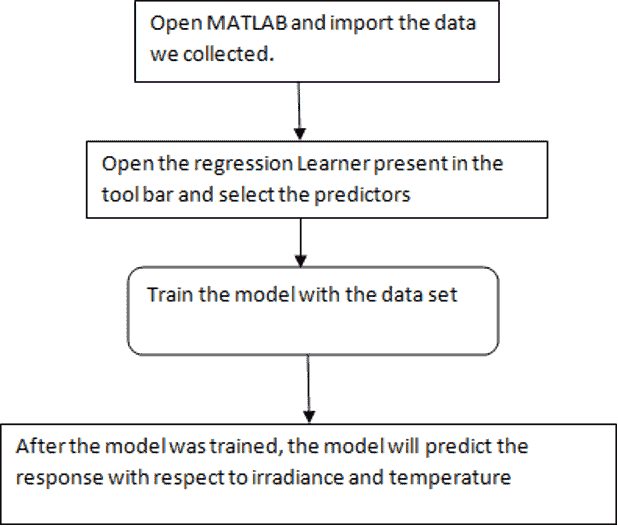
Fig 6.1.1 Flow Chart
6.2 PROCEDURE FOR ANALYSIS OF ANALYSIS OF 30KW SOLAR PV SYSTEM USING MACHINE LEARNING
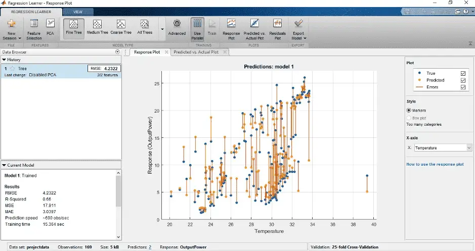
In this project linear regression is carried out in MATLAB. The step-by-step procedure to predict and analyze the performance using the data we collected (i.e) Irradiance, Temperature, and Output power.
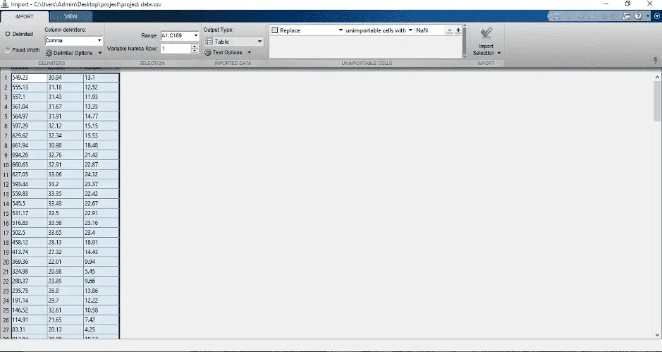
Step 1: Open the MATLAB software and we have to import the data collected in .csv format by clicking the import data.
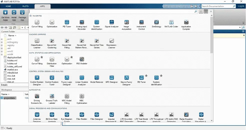
Step 2: Open the “regression learner” from apps present in the toolbar.
Step 3: A new tab will open. Click “new session” present in the toolbar.

Step 4: We have to select the predictors and the response (dependant variable)
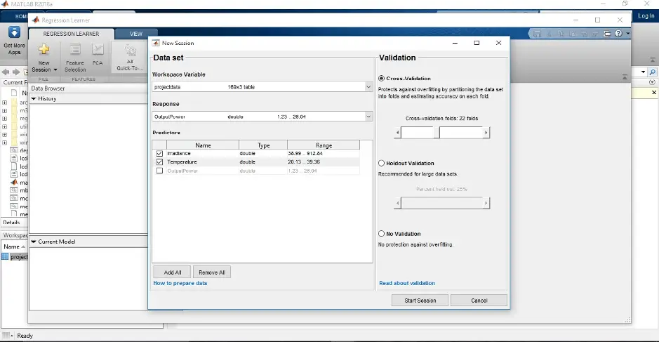
Step 5: With the data we uploaded, train the model.
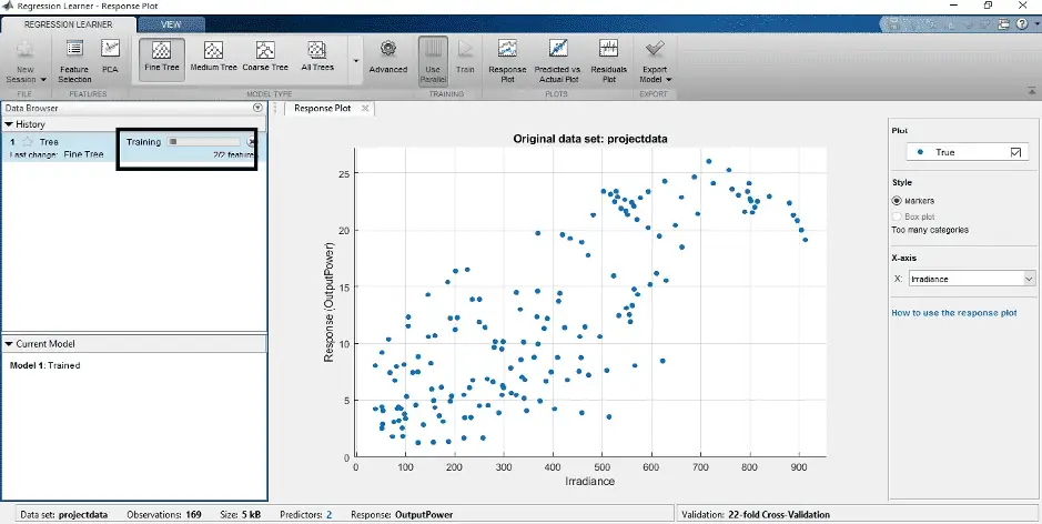
Step 6: we can also check the error using predictor vs. actual plot. If the error is small then all points are lying almost close to the line.
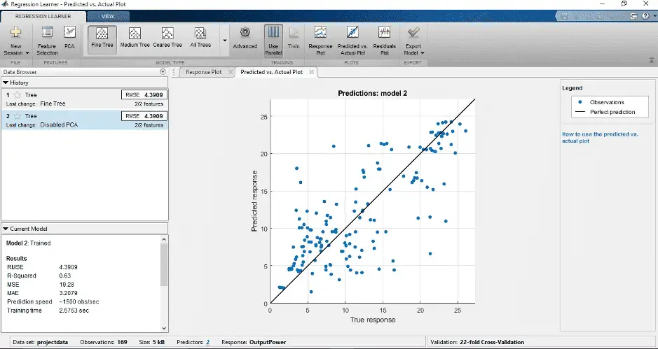
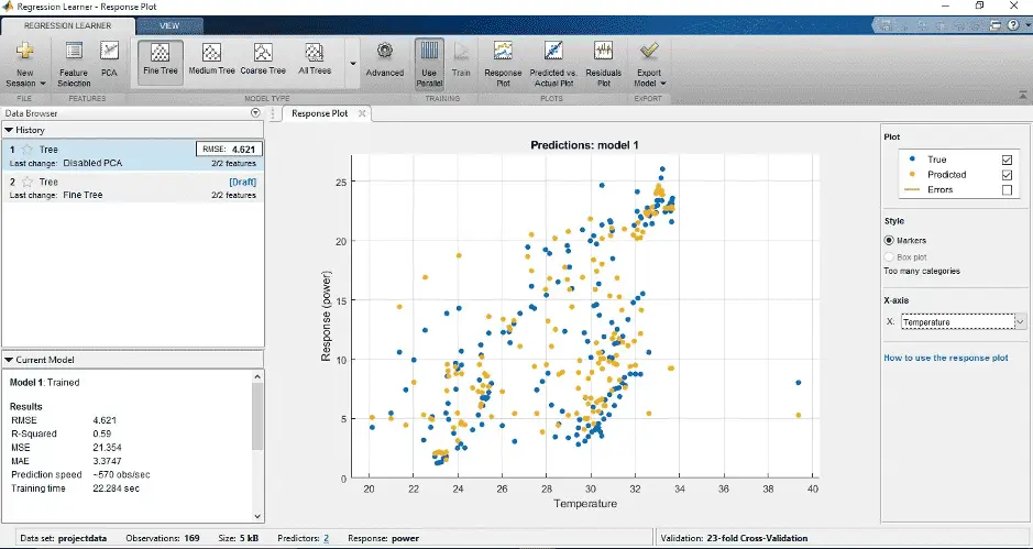
Step 7: After the model was trained, the model will predict the response(here output power) for the data we gave concerning Irradiance and Temperature.
Temperature VS Output power
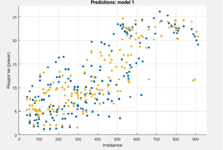
Irradiance VS Output Power
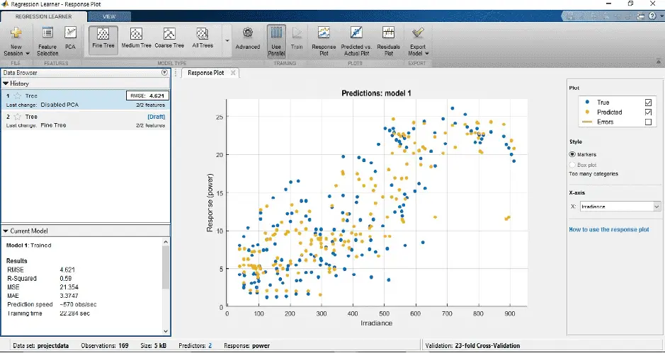
Step 8: We can see the error between the predicted value and the true value in the graph.
7 CONCLUSION AND FUTURE WORK
7.1 CONCLUSION FOR ANALYSIS OF 30KW SOLAR PV SYSTEM
The major challenge in solar energy generation is the volatility intermittent of photovoltaic system power generation due mainly to weather conditions. Thus, accurate forecasting of photovoltaic power generation is becoming indispensable for reducing the effect of uncertainty and energy costs and enabling suitable integration of photovoltaic systems in a smart grid. In this project, for the data set required to train the model Output power is collected from the inverter of the 30kW solar PV system installed on our campus. Irradiance and Temperature were collected from NASA with data on the same dates as output power was collected. With the data set, the model is trained in MATLAB using a linear regression algorithm. After the model was trained it gave predicted value to the input (predictors) we gave.
7.1.1 RESULTS: Irradiance VS Output power
Temperature VS Output Power
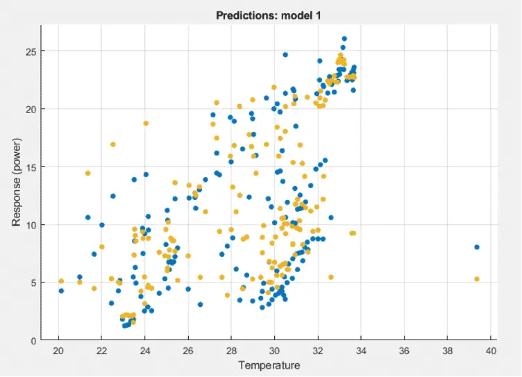
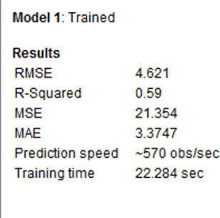
Here the blue dots represent actual value and yellow dots represent predicted value. The result from the predicted model is shown in fig 7.1.1.3
7.2 FUTURE WORK
In our project, nearly 60% of the efficiency is achieved. In the future, we will increase efficiency by increasing the number of data required for training and implementing different machine learning techniques.
REFERENCE
- https://sci-hub.hkvisa.net/10.1016/j.rser.2014.12.031
- https://www.geeksforgeeks.org/ml-advantages-and-disadvantages-of-linear- regression/
- https://machinelearningmastery.com/linear-regression-for- machine-learning/
- https://energyeducation.ca/encyclopedia/Photovoltaic_system
- https://www.sciencedirect.com/science/article/abs/pii/S13640321 14010831
- www.morganclaypoolpublishers.com
- https://www.sciencedirect.com/science/article/abs/pii/S15684946 14005857
- Https://machinelearningmastery.com/basic-concepts-in-machine- learning/
- www.genusinnovation.com
- https://power.larc.nasa.gov/data-access-viewer/
- https://towardsdatascience.com/linear-regression-detailed-view-ea73175f6e86
- A Review on Linear Regression Comprehensive in Machine Learning Dastan Hussen Maulud1, * , Adnan Mohsin Abdulazeez (2020)https://jastt.org/index.php/jasttpath/article/download/57/20
- Solar photovoltaic power output forecasting using machine learning technique ; Dinh Van Tai 2019 J. Phys.: Conf. Ser. 1327 012051
- Mehrbakhsh Nilashi, Othman bin Ibrahim, Hossein Ahmadi, Leila Shahmoradi An analytical method for diseases prediction using machine learning techniques, Computers & Chemical Engineering, Volume 106, 2017, Pages 212-223, ISSN 0098-1354,https://doi.org/10.1016/j.compchemeng.2017.06.011.
- Modeling, simulation and performance analysis of solar PV array configurations (Series, Series–Parallel and Honey-Comb) to extract maximum power under Partial Shading Conditions; Suneel Raju Penderm, Suresh Mikkili(2021)https://www.sciencedirect.com/science/article/pii/S2352484717302378
- A. Khosravi, R.N.N. Koury, L. Machado, J.J.G. Pabon, Prediction of hourly solar radiation in Abu Musa Island using machine learning algorithms, Journal of Cleaner Production,Volume 176, 2018, Pages 63-75, ISSN 0959- 6526,https://doi.org/10.1016/j.jclepro.2017.12.065.
- Modeling and performance analysis of a solar PV power system under irradiation and load variations;F. E. Tahiri , Khalid Chikh, Mohamed Khafallah (2018)https://ieeexplore.ieee.org/abstract/document/8166952
Credit: This Project “Prediction And Performance Analysis Of 30kW Solar Pv System Using Machine Learning Linear Regression Algorithm” was completed by KRITHIKAA KK, KOWSIKA NP, and HARSHA M under the supervision of Mr.S.Balamurugan and Dr. K. BASKARAN (HOD) from the Department of Electrical And Electronics Engineering of Alagappa Chettiar Government College Of Engineering And Technology karaikudi.

Leave a Reply